Running inference on MXNet/Gluon from an ONNX model
Open Neural Network Exchange (ONNX) provides an open source format for AI models. It defines an extensible computation graph model, as well as definitions of built-in operators and standard data types.
In this tutorial we will:
learn how to load a pre-trained .onnx model file into MXNet/Gluon
learn how to test this model using the sample input/output
learn how to test the model on custom images
Pre-requisite
To run the tutorial you will need to have installed the following python modules: - MXNet > 1.1.0 - onnx (follow the install guide) - matplotlib
import numpy as np
import mxnet as mx
from mxnet.contrib import onnx as onnx_mxnet
from mxnet import gluon, nd
%matplotlib inline
import matplotlib.pyplot as plt
import tarfile, os
import json
import logging
logging.basicConfig(level=logging.INFO)
Downloading supporting files
These are images and a vizualisation script
image_folder = "images"
utils_file = "utils.py" # contain utils function to plot nice visualization
image_net_labels_file = "image_net_labels.json"
images = ['apron.jpg', 'hammerheadshark.jpg', 'dog.jpg', 'wrench.jpg', 'dolphin.jpg', 'lotus.jpg']
base_url = "https://raw.githubusercontent.com/dmlc/web-data/master/mxnet/doc/tutorials/onnx/{}?raw=true"

for image in images:
    mx.test_utils.download(base_url.format("{}/{}".format(image_folder, image)), fname=image,dirname=image_folder)
mx.test_utils.download(base_url.format(utils_file), fname=utils_file)
mx.test_utils.download(base_url.format(image_net_labels_file), fname=image_net_labels_file)

from utils import *
Downloading a model from the ONNX model zoo
We download a pre-trained model, in our case the GoogleNet model, trained on ImageNet from the ONNX model zoo. The model comes packaged in an archive tar.gz file containing an model.onnx model file.
base_url = "https://s3.amazonaws.com/download.onnx/models/opset_3/"
current_model = "bvlc_googlenet"
model_folder = "model"
archive = "{}.tar.gz".format(current_model)
archive_file = os.path.join(model_folder, archive)
url = "{}{}".format(base_url, archive)
Download and extract pre-trained model
mx.test_utils.download(url, dirname = model_folder)
if not os.path.isdir(os.path.join(model_folder, current_model)):
    print('Extracting model...')
    tar = tarfile.open(archive_file, "r:gz")
    tar.extractall(model_folder)
    tar.close()
    print('Extracted')
The models have been pre-trained on ImageNet, let’s load the label mapping of the 1000 classes.
categories = json.load(open(image_net_labels_file, 'r'))
Loading the model into MXNet Gluon
onnx_path = os.path.join(model_folder, current_model, "model.onnx")
We get the symbol and parameter objects
sym, arg_params, aux_params = onnx_mxnet.import_model(onnx_path)
We pick a context, CPU is fine for inference, switch to mx.gpu() if you want to use your GPU.
ctx = mx.cpu()
We obtain the data names of the inputs to the model by using the model metadata API:
model_metadata = onnx_mxnet.get_model_metadata(onnx_path)
print(model_metadata)
{'output_tensor_data': [(u'gpu_0/softmax_1', (1L, 1000L))],
 'input_tensor_data': [(u'gpu_0/data_0', (1L, 3L, 224L, 224L))]}
data_names = [inputs[0] for inputs in model_metadata.get('input_tensor_data')]
print(data_names)
And load them into a MXNet Gluon symbol block.

```python
import warnings
with warnings.catch_warnings():
    warnings.simplefilter("ignore")
    net = gluon.nn.SymbolBlock(outputs=sym, inputs=mx.sym.var('data_0'))
net_params = net.collect_params()
for param in arg_params:
    if param in net_params:
        net_params[param]._load_init(arg_params[param], ctx=ctx)
for param in aux_params:
    if param in net_params:
        net_params[param]._load_init(aux_params[param], ctx=ctx)
We can now cache the computational graph through hybridization to gain some performance
net.hybridize()
We can visualize the network (requires graphviz installed)
mx.visualization.plot_network(sym, node_attrs={"shape":"oval","fixedsize":"false"})
This is a helper function to run M batches of data of batch-size N through the net and collate the outputs into an array of shape (K, 1000) where K=MxN is the total number of examples (mumber of batches x batch-size) run through the network.
def run_batch(net, data):
    results = []
    for batch in data:
        outputs = net(batch)
        results.extend([o for o in outputs.asnumpy()])
    return np.array(results)
Test using real images
TOP_P = 3 # How many top guesses we show in the visualization
Transform function to set the data into the format the network expects, (N, 3, 224, 224) where N is the batch size.
def transform(img):
    return np.expand_dims(np.transpose(img, (2,0,1)),axis=0).astype(np.float32)
We load two sets of images in memory
image_net_images = [plt.imread('{}/{}.jpg'.format(image_folder, path)) for path in ['apron', 'hammerheadshark','dog']]
caltech101_images = [plt.imread('{}/{}.jpg'.format(image_folder, path)) for path in ['wrench', 'dolphin','lotus']]
images = image_net_images + caltech101_images
And run them as a batch through the network to get the predictions
batch = nd.array(np.concatenate([transform(img) for img in images], axis=0), ctx=ctx)
result = run_batch(net, [batch])
plot_predictions(image_net_images, result[:3], categories, TOP_P)
Well done! Looks like it is doing a pretty good job at classifying pictures when the category is a ImageNet label
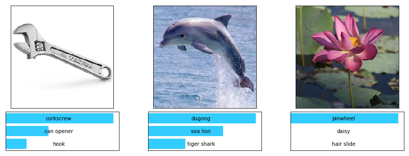
Let’s now see the results on the 3 other images
plot_predictions(caltech101_images, result[3:7], categories, TOP_P)
Hmm, not so good… Even though predictions are close, they are not accurate, which is due to the fact that the ImageNet dataset does not contain wrench, dolphin, or lotus categories and our network has been trained on ImageNet.
Lucky for us, the Caltech101 dataset has them, let’s see how we can fine-tune our network to classify these categories correctly.
We show that in our next tutorial: