Visualizing Decisions of Convolutional Neural Networks
Convolutional Neural Networks have made a lot of progress in Computer Vision. Their accuracy is as good as humans in some tasks. However it remains hard to explain the predictions of convolutional neural networks, as they lack the interpretability offered by other models, for example decision trees.
It is often helpful to be able to explain why a model made the prediction it made. For example when a model misclassifies an image, it is hard to say why without visualizing the network’s decision.
Visualizations also help build confidence about the predictions of a model. For example, even if a model correctly predicts birds as birds, we would want to confirm that the model bases its decision on the features of bird and not on the features of some other object that might occur together with birds in the dataset (like leaves).
In this tutorial, we show how to visualize the predictions made by convolutional neural networks using Gradient-weighted Class Activation Mapping. Unlike many other visualization methods, Grad-CAM can be used on a wide variety of CNN model families - CNNs with fully connected layers, CNNs used for structural outputs (e.g. captioning), CNNs used in tasks with multi-model input (e.g. VQA) or reinforcement learning without architectural changes or re-training.
In the rest of this notebook, we will explain how to visualize predictions made by VGG-16. We begin by importing the required dependencies. gradcam module contains the implementation of visualization techniques used in this notebook.
from __future__ import print_function

import mxnet as mx
from mxnet import gluon

from matplotlib import pyplot as plt
import numpy as np

gradcam_file = "gradcam.py"
base_url = "https://raw.githubusercontent.com/indhub/mxnet/cnnviz/example/cnn_visualization/{}?raw=true"
mx.test_utils.download(base_url.format(gradcam_file), fname=gradcam_file)
import gradcam
Building the network to visualize
Next, we build the network we want to visualize. For this example, we will use the VGG-16 network. This code was taken from the Gluon model zoo and refactored to make it easy to switch between gradcam‘s and Gluon’s implementation of ReLU and Conv2D. Same code can be used for both training and visualization with a minor (one line) change.
Notice that we import ReLU and Conv2D from gradcam module instead of mxnet.gluon.nn.
- We use a modified ReLU because we use guided backpropagation for visualization and guided backprop requires ReLU layer to block the backward flow of negative gradients corresponding to the neurons which decrease the activation of the higher layer unit we aim to visualize. Check this paper to learn more about guided backprop.
- We use a modified Conv2D (a wrapper on top of Gluon’s Conv2D) because we want to capture the output of a given convolutional layer and its gradients. This is needed to implement Grad-CAM. Check this paper to learn more about Grad-CAM.
When you train the network, you could just import Activation and Conv2D from gluon.nn instead. No other part of the code needs any change to switch between training and visualization.
import os
from mxnet.gluon.model_zoo import model_store

from mxnet.initializer import Xavier
from mxnet.gluon.nn import MaxPool2D, Flatten, Dense, Dropout, BatchNorm
from gradcam import Activation, Conv2D

class VGG(mx.gluon.HybridBlock):
    def __init__(self, layers, filters, classes=1000, **kwargs):
        super(VGG, self).__init__(**kwargs)
        assert len(layers) == len(filters)
        with self.name_scope():
            self.features = self._make_features(layers, filters)
            self.features.add(Dense(4096, activation='relu',
                                       weight_initializer='normal',
                                       bias_initializer='zeros'))
            self.features.add(Dropout(rate=0.5))
            self.features.add(Dense(4096, activation='relu',
                                       weight_initializer='normal',
                                       bias_initializer='zeros'))
            self.features.add(Dropout(rate=0.5))
            self.output = Dense(classes,
                                   weight_initializer='normal',
                                   bias_initializer='zeros')

    def _make_features(self, layers, filters):
        featurizer = mx.gluon.nn.HybridSequential(prefix='')
        for i, num in enumerate(layers):
            for _ in range(num):
                featurizer.add(Conv2D(filters[i], kernel_size=3, padding=1,
                                         weight_initializer=Xavier(rnd_type='gaussian',
                                                                   factor_type='out',
                                                                   magnitude=2),
                                         bias_initializer='zeros'))
                featurizer.add(Activation('relu'))
            featurizer.add(MaxPool2D(strides=2))
        return featurizer

    def hybrid_forward(self, F, x):
        x = self.features(x)
        x = self.output(x)
        return x
Loading pretrained weights
We’ll use pre-trained weights (trained on ImageNet) from model zoo instead of training the model from scratch.
# Number of convolution layers and number of filters for each VGG configuration.
# Check the VGG [paper](https://arxiv.org/abs/1409.1556) for more details on the different architectures.
vgg_spec = {11: ([1, 1, 2, 2, 2], [64, 128, 256, 512, 512]),
            13: ([2, 2, 2, 2, 2], [64, 128, 256, 512, 512]),
            16: ([2, 2, 3, 3, 3], [64, 128, 256, 512, 512]),
            19: ([2, 2, 4, 4, 4], [64, 128, 256, 512, 512])}

def get_vgg(num_layers, ctx=mx.cpu(), root=os.path.join('~', '.mxnet', 'models'), **kwargs):

    # Get the number of convolution layers and filters
    layers, filters = vgg_spec[num_layers]

    # Build the VGG network
    net = VGG(layers, filters, **kwargs)

    # Load pretrained weights from model zoo
    from mxnet.gluon.model_zoo.model_store import get_model_file
    net.load_params(get_model_file('vgg%d' % num_layers, root=root), ctx=ctx)

    return net

def vgg16(**kwargs):
    return get_vgg(16, **kwargs)
Preprocessing and other helpers
We’ll resize the input image to 224x224 before feeding it to the network. We normalize the images using the same parameters ImageNet dataset was normalised using to create the pretrained model. These parameters are published here. We use transpose to convert the image to channel-last format.
Note that we do not hybridize the network. This is because we want gradcam.Activation and gradcam.Conv2D to behave differently at different times during the execution. For example, gradcam.Activation will do the regular backpropagation while computing the gradient of the topmost convolutional layer but will do guided backpropagation when computing the gradient of the image.
image_sz = (224, 224)

def preprocess(data):
    data = mx.image.imresize(data, image_sz[0], image_sz[1])
    data = data.astype(np.float32)
    data = data/255
    data = mx.image.color_normalize(data,
                                    mean=mx.nd.array([0.485, 0.456, 0.406]),
                                    std=mx.nd.array([0.229, 0.224, 0.225]))
    data = mx.nd.transpose(data, (2,0,1))
    return data

network = vgg16(ctx=mx.cpu())
We define a helper to display multiple images in a row in Jupyter notebook.
def show_images(pred_str, images):
    titles = [pred_str, 'Grad-CAM', 'Guided Grad-CAM', 'Saliency Map']
    num_images = len(images)
    fig=plt.figure(figsize=(15,15))
    rows, cols = 1, num_images
    for i in range(num_images):
        fig.add_subplot(rows, cols, i+1)
        plt.xlabel(titles[i])
        plt.imshow(images[i], cmap='gray' if i==num_images-1 else None)
    plt.show()
Given an image, the network predicts a probability distribution over all categories. The most probable category can be found by applying the argmax operation. This gives an integer corresponding to the category. We still need to convert this to a human readable category name to know what category the network predicted. Synset file contains the mapping between Imagenet category index and category name. We’ll download the synset file, load it in a list to convert category index to human readable category names.
synset_url = "http://data.mxnet.io/models/imagenet/synset.txt"
synset_file_name = "synset.txt"
mx.test_utils.download(synset_url, fname=synset_file_name)
synset = []
with open('synset.txt', 'r') as f:
    synset = [l.rstrip().split(' ', 1)[1].split(',')[0] for l in f]

def get_class_name(cls_id):
    return "%s (%d)" % (synset[cls_id], cls_id)

def run_inference(net, data):
    out = net(data)
    return out.argmax(axis=1).asnumpy()[0].astype(int)
Visualizing CNN decisions
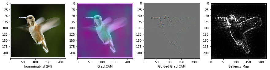
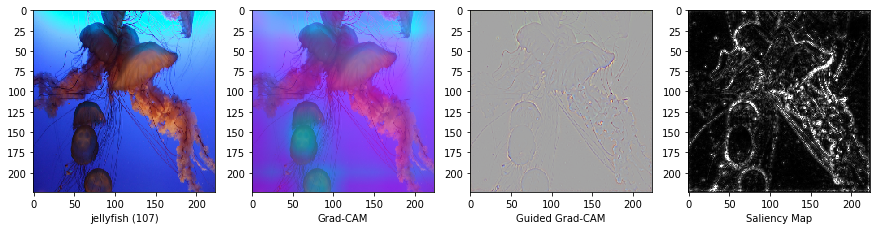
Next, we’ll write a method to get an image, preprocess it, predict category and visualize the prediction. We’ll use gradcam.visualize() to create the visualizations. gradcam.visualize returns a tuple with the following visualizations:
- Grad-CAM: This is a heatmap superimposed on the input image showing which part(s) of the image contributed most to the CNN’s decision.
- Guided Grad-CAM: Guided Grad-CAM shows which exact pixels contributed the most to the CNN’s decision.
- Saliency map: Saliency map is a monochrome image showing which pixels contributed the most to the CNN’s decision. Sometimes, it is easier to see the areas in the image that most influence the output in a monochrome image than in a color image.
def visualize(net, img_path, conv_layer_name):
    orig_img = mx.img.imread(img_path)
    preprocessed_img = preprocess(orig_img)
    preprocessed_img = preprocessed_img.expand_dims(axis=0)

    pred_str = get_class_name(run_inference(net, preprocessed_img))

    orig_img = mx.image.imresize(orig_img, image_sz[0], image_sz[1]).asnumpy()
    vizs = gradcam.visualize(net, preprocessed_img, orig_img, conv_layer_name)
    return (pred_str, (orig_img, *vizs))
Next, we need to get the name of the last convolutional layer that extracts features from the image. We use the gradient information flowing into the last convolutional layer of the CNN to understand the importance of each neuron for a decision of interest. We are interested in the last convolutional layer because convolutional features naturally retain spatial information which is lost in fully connected layers. So, we expect the last convolutional layer to have the best compromise between high level semantics and detailed spacial information. The neurons in this layer look for semantic class specific information in the image (like object parts).
In our network, feature extractors are added to a HybridSequential block named features. You can list the layers in that block by just printing network.features. You can see that the topmost convolutional layer is at index 28. network.features[28]._name will give the name of the layer.
last_conv_layer_name = network.features[28]._name
print(last_conv_layer_name)
vgg0_conv2d12
Let’s download some images we can use for visualization.
images = ["hummingbird.jpg", "jellyfish.jpg", "snow_leopard.jpg", "volcano.jpg"]
base_url = "https://raw.githubusercontent.com/dmlc/web-data/master/mxnet/example/cnn_visualization/{}?raw=true"
for image in images:
    mx.test_utils.download(base_url.format(image), fname=image)
We now have everything we need to start visualizing. Let’s visualize the CNN decision for the images we downloaded.
show_images(*visualize(network, "hummingbird.jpg", last_conv_layer_name))
show_images(*visualize(network, "jellyfish.jpg", last_conv_layer_name))
show_images(*visualize(network, "snow_leopard.jpg", last_conv_layer_name))
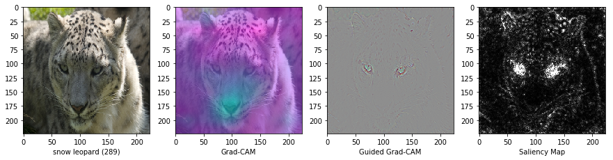
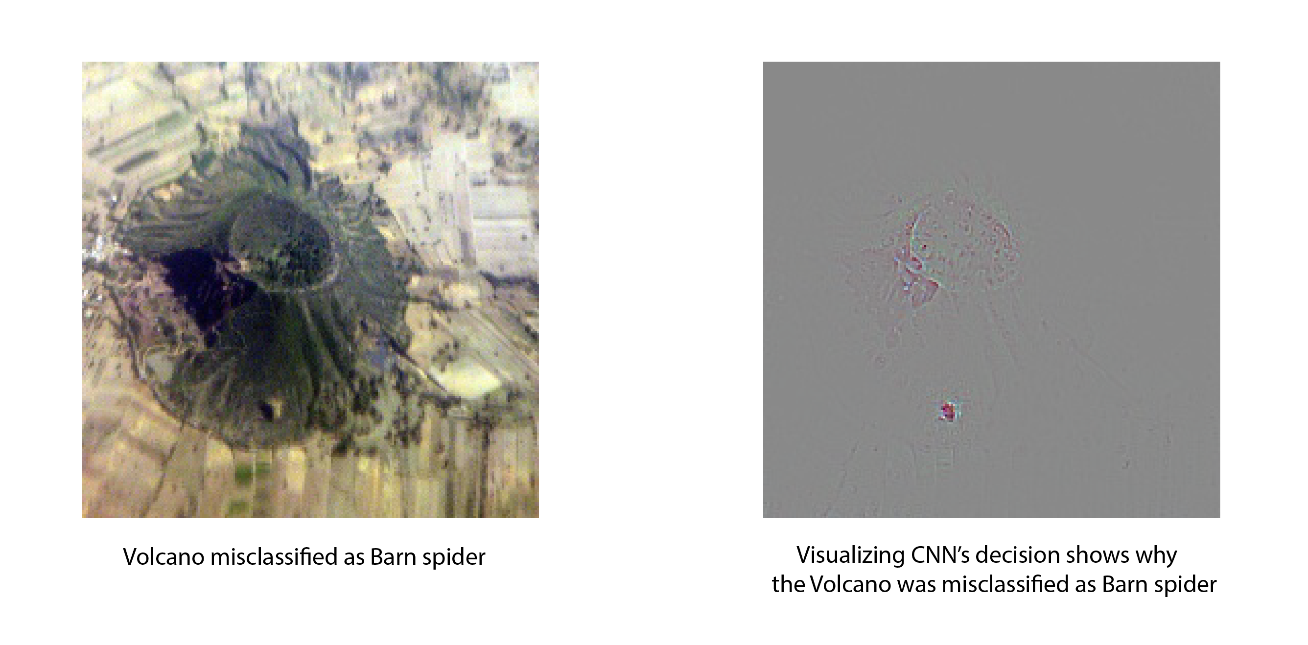
Shown above are some images the network was able to predict correctly. We can see that the network is basing its decision on the appropriate features. Now, let’s look at an example that the network gets the prediction wrong and visualize why it gets the prediction wrong.
show_images(*visualize(network, "volcano.jpg", last_conv_layer_name))
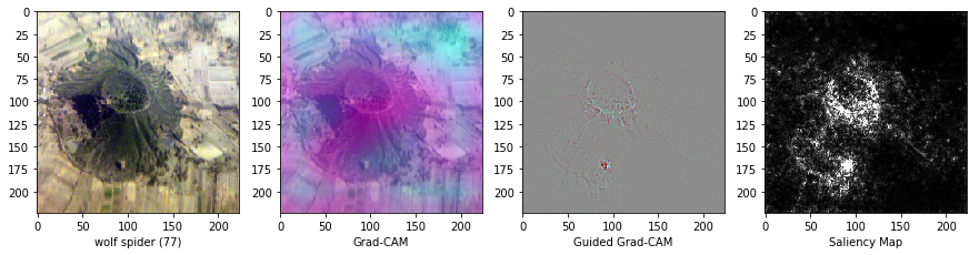
While it is not immediately evident why the network thinks this volcano is a spider, after looking at the Grad-CAM visualization, it is hard to look at the volcano and not see the spider!
Being able to visualize why a CNN predicts specific classes is a powerful tool to diagnose prediction failures. Even when the network is making correct predictions, visualizing activations is an important step to verify that the network is making its decisions based on the right features and not some correlation which happens to exist in the training data.
The visualization method demonstrated in this tutorial applies to a wide variety of network architectures and a wide variety of tasks beyond classification - like VQA and image captioning. Any type of differentiable output can be used to create the visualizations shown above. Visualization techniques like these solve (at least partially) the long standing problem of interpretability of neural networks.