Large Scale Image Classification
Training a neural network with a large number of images presents several challenges. Even with the latest GPUs, it is not possible to train large networks using a large number of images in a reasonable amount of time using a single GPU. This problem can be somewhat mitigated by using multiple GPUs in a single machine. But there is a limit to the number of GPUs that can be attached to one machine (typically 8 or 16). This tutorial explains how to train large networks with terabytes of data using multiple machines each containing multiple GPUs.
Prerequisites
- MXNet. See the instructions for your operating system in Setup and Installation.
- OpenCV Python library
$ pip install opencv-python
Preprocessing
Disk space
The first step in training with large data is downloading the data and preprocessing it. For this tutorial, we will be using the full ImageNet dataset. Note that, at least 2 TB of disk space is required to download and preprocess this data. It is strongly recommended to use SSD instead of HDD. SSD is much better at dealing with a large number of small image files. After the preprocessing completes and images are packed into recordIO files, HDD should be fine for training.
In this tutorial, we will use an AWS storage instance for data preprocessing. The storage instance i3.4xlarge has 3.8 TB of disk space across two NVMe SSD disks. We will use software RAID to combine them into one disk and mount it at ~/data.
sudo mdadm --create --verbose /dev/md0 --level=stripe --raid-devices=2 \
    /dev/nvme0n1 /dev/nvme1n1
sudo mkfs /dev/md0
sudo mkdir ~/data
sudo mount /dev/md0 ~/data
sudo chown ${whoami} ~/data
We now have sufficient disk space to download and preprocess the data.
Download ImageNet
In this tutorial, we will be using the full ImageNet dataset which can be downloaded from http://www.image-net.org/download-images. fall11_whole.tar contains all the images. This file is 1.2 TB in size and could take a long time to download.
After downloading, untar the file.
export ROOT=full
mkdir $ROOT
tar -xvf fall11_whole.tar -C $ROOT
That should give you a collection of tar files. Each tar file represents a category and contains all images belonging to that category. We can unzip each tar file and copy the images into a folder named after the name of the tar file.
for i in $ROOT/*.tar; do j=${i%.*}; echo $j;  mkdir -p $j; tar -xf $i -C $j; done
rm $ROOT/*.tar

ls $ROOT | head
n00004475
n00005787
n00006024
n00006484
n00007846
n00015388
n00017222
n00021265
n00021939
n00120010
Remove uncommon classes for transfer learning (optional)
A common reason to train a network on ImageNet data is to use it for transfer learning (including feature extraction or fine-tuning other models). According to this study, classes with too few images don’t help in transfer learning. So, we could remove classes with fewer than a certain number of images. The following code will remove classes with less than 500 images.
BAK=${ROOT}_filtered
mkdir -p ${BAK}
for c in ${ROOT}/n*; do
    count=`ls $c/*.JPEG | wc -l`
    if [ "$count" -gt "500" ]; then
        echo "keep $c, count = $count"
    else
        echo "remove $c, $count"
        mv $c ${BAK}/
    fi
done
Generate a validation set
To ensure we don’t overfit the data, we will create a validation set separate from the training set. During training, we will monitor loss on the validation set frequently. We create the validation set by picking fifty random images from each class and moving them to the validation set.
VAL_ROOT=${ROOT}_val
mkdir -p ${VAL_ROOT}
for i in ${ROOT}/n*; do
    c=`basename $i`
    echo $c
    mkdir -p ${VAL_ROOT}/$c
    for j in `ls $i/*.JPEG | shuf | head -n 50`; do
        mv $j ${VAL_ROOT}/$c/
    done
done
Pack images into record files
While MXNet can read image files directly, it is recommended to pack the image files into a recordIO file for increased performance. MXNet provides a tool (tools/im2rec.py) to do this. To use this tool, MXNet and OpenCV’s python module needs to be installed in the system.
Set the environment variable MXNET to point to the MXNet installation directory and NAME to the name of the dataset. Here, we assume MXNet is installed at ~/mxnet
MXNET=~/mxnet
NAME=full_imagenet_500_filtered
To create the recordIO files, we first create a list of images we want in the recordIO files and then use im2rec to pack images in the list into recordIO files. We create this list in train_meta. Training data is around 1TB. We split it into 8 parts, with each part roughly 100 GB in size.
mkdir -p train_meta
python ${MXNET}/tools/im2rec.py --list --chunks 8 --recursive \
train_meta/${NAME} ${ROOT}
We then resize the images such that the short edge is 480 pixels long and pack the images into recordIO files. Since most of the work is disk I/O, we use multiple (16) threads to get the work done faster.
python ${MXNET}/tools/im2rec.py --resize 480 --quality 90 \
--num-thread 16 train_meta/${NAME} ${ROOT}
Once done, we move the rec files into a folder named train.
mkdir -p train
mv train_meta/*.rec train/
We do similar preprocessing for the validation set.
mkdir -p val_meta
python ${MXNET}/tools/im2rec.py --list --recursive \
val_meta/${NAME} ${VAL_ROOT}
python ${MXNET}/tools/im2rec.py --resize 480 --quality 90 \
--num-thread 16 val_meta/${NAME} ${VAL_ROOT}
mkdir -p val
mv val_meta/*.rec val/
We now have all training and validation images in recordIO format in train and val directories respectively. We can now use these .rec files for training.
Training
ResNet has shown its effectiveness on ImageNet competition. Our experiments also reproduced the results reported in the paper. As we increase the number of layers from 18 to 152, we see steady improvement in validation accuracy. Given this is a huge dataset, we will use Resnet with 152 layers.
Due to the huge computational complexity, even the fastest GPU needs more than one day for a single pass of the data. We often need tens of epochs before the training converges to good validation accuracy. While we can use multiple GPUs in a machine, the number of GPUs in a machine is often limited to 8 or 16. For faster training, in this tutorial, we will use multiple machines each containing multiple GPUs to train the model.
Setup
We will use 16 machines (P2.16x instances), each containing 16 GPUs (Tesla K80). These machines are interconnected via 20 Gbps ethernet.
AWS CloudFormation makes it very easy to create deep learning clusters. We follow instructions from this page and create a deep learning cluster with 16 P2.16x instances.
We load the data and code in the first machine (we’ll refer to this machine as master). We share both the data and code to other machines using EFS.
If you are setting up your cluster manually, without using AWS CloudFormation, remember to do the following:
Compile MXNet using
USE_DIST_KVSTORE=1to enable distributed training.Create a hosts file in the master that contains the host names of all the machines in the cluster. For example,
$ head -3 hosts
deeplearning-worker1
deeplearning-worker2
deeplearning-worker3
It should be possible to ssh into any of these machines from the master by invoking
sshwith just a hostname from the file. For example,$ ssh deeplearning-worker2 =================================== Deep Learning AMI for Ubuntu =================================== ... ubuntu@ip-10-0-1-199:~$
One way to do this is to use ssh agent forwarding. Please check this page to learn how to set this up. In short, you’ll configure all machines to login using a particular certificate (mycert.pem) which is present on your local machine. You then login to the master using the certificate and the
-Aswitch to enable agent forwarding. Now, from the master, you should be able to login to any other machine in the cluster by providing just the hostname (example:ssh deeplearning-worker2).
Run Training
After the cluster is setup, login to master and run the following command from ${MXNET}/example/image-classification
../../tools/launch.py -n 16 -H $DEEPLEARNING_WORKERS_PATH python train_imagenet.py --network resnet \
--num-layers 152 --data-train ~/data/train --data-val ~/data/val/ --gpus 0,1,2,3,4,5,6,7,8,9,10,11,12,13,14,15 \
--batch-size 8192 --model ~/data/model/resnet152 --num-epochs 1 --kv-store dist_sync
launch.py launches the command it is provided in all the machine in the cluster. List of machines in the cluster must be provided to launch.py using the -H switch. Here is description of options used for launch.py.
| Option | Description |
|---|---|
| n | specifies the number of worker jobs to run on each machine. We run 16 workers since we have 16 machines in the cluster. |
| H | specifies the path to a file that has a list of hostnames of machines in the cluster. Since we created the cluster using the AWS deep learning CloudFormation template, the environment variable $DEEPLEARNING_WORKERS_PATH points to the required file. |
train_imagenet.py trains the network provided by the --network option using the data provided by the --data-train and --data-val options. Here is description of the options used with train_imagenet.py.
| Option | Description |
|---|---|
| network | The network to train. Could be any of the network available in ${MXNET}/example/image-classification. For this tutorial, we use Resnet. |
| num-layers | Number of layers to use in the network. We use 152 layer Resnet. |
| data-train | Directory containing the training images. We point to the EFS location (~/data/train/) where we stored the training images. |
| data-val | Directory containing the validation images. We point to the EFS location (~/data/val) where we stored the validation images. |
| gpus | Comma separated list of gpu indices to use for training on each machine. We use all 16 GPUs. |
| batch-size | Batch size across all GPUs. This is equal to batch size per GPU * total number of GPUs. We use a batch size of 32 images per GPU. So, effective batch size is 32 * 16 * 16 = 8192. |
| model | Path prefix for the model file created by the training. |
| num-epochs | Number of epochs to train. |
| kv-store | Key/Value store for parameter synchronization. We use distributed kv store since we are doing distributed training. |
After training is complete, trained models are available in the directory specified by the --model option. Models are saved in two parts: model-symbol.json for the network definition and model-n.params for the parameters saved after the n’th epoch.
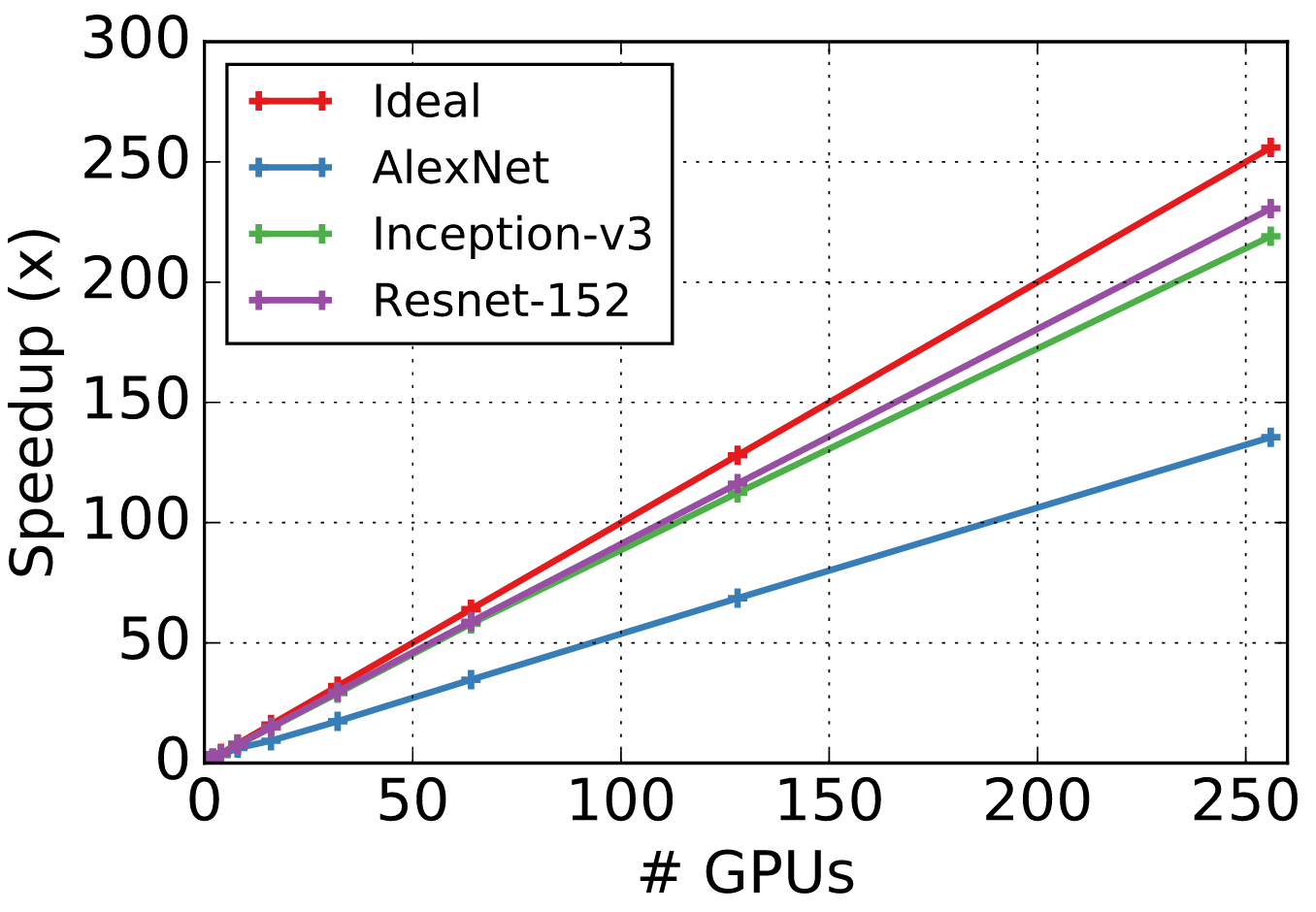
Scalability
One common concern using large number of machines for training is the scalability. We have benchmarked scalability running several popular networks on clusters with up to 256 GPUs and the speedup is very close to ideal.
This scalability test was run on sixteen P2.16xl instances with 256 GPUs in total. We used AWS deep learning AMI with CUDA 7.5 and CUDNN 5.1 installed.
We fixed the batch size per GPU constant and doubled the number of GPUs for every subsequent test. Synchronized SGD (–kv-store dist_device_sync) was used. The CNNs used are located here.
| alexnet | inception-v3 | resnet-152 | |
|---|---|---|---|
| batch size per GPU | 512 | 32 | 32 |
| model size (MB) | 203 | 95 | 240 |
Number of images processed per second is shown in the following table:
| Number of GPUs | Alexnet | Inception-v3 | Resnet-152 |
|---|---|---|---|
| 1 | 457.07 | 30.4 | 20.8 |
| 2 | 870.43 | 59.61 | 38.76 |
| 4 | 1514.8 | 117.9 | 77.01 |
| 8 | 2852.5 | 233.39 | 153.07 |
| 16 | 4244.18 | 447.61 | 298.03 |
| 32 | 7945.57 | 882.57 | 595.53 |
| 64 | 15840.52 | 1761.24 | 1179.86 |
| 128 | 31334.88 | 3416.2 | 2333.47 |
| 256 | 61938.36 | 6660.98 | 4630.42 |
The following figure shows speedup against the number of GPUs used and compares it with ideal speedup.
Troubleshooting guidelines
Validation accuracy
It is often straightforward to achieve a reasonable validation accuracy, but achieving the state-of-the-art numbers reported in papers can sometimes be very hard. Here are few things you can try to improve validation accuracy.
- Adding more data augmentations often reduces the gap between training and validation accuracy. Data augmentation could be reduced in epochs closer to the end.
- Start with a large learning rate and keep it large for a long time. For example, in CIFAR10, you could keep the learning rate at 0.1 for the first 200 epochs and then reduce it to 0.01.
- Do not use a batch size that is too large, especially batch size >> number of classes.
Speed
- Distributed training improves speed when computation cost of a batch is high. So, make sure your workload is not too small (like LeNet on MNIST). Make sure batch size is reasonably large.
- Make sure data-read and preprocessing is not the bottleneck. Use the
--test-io 1flag to check how many images can be pre-processed per second. - Increase –data-nthreads (default is 4) to use more threads for data preprocessing.
- Data preprocessing is done by opencv. If opencv is compiled from source code, check if it is configured correctly.
- Use
--benchmark 1to use randomly generated data rather than real data to narrow down where the bottleneck is. - Check this page for more details.
Memory
If the batch size is too big, it can exhaust GPU memory. If this happens, you’ll see the error message “cudaMalloc failed: out of memory” or something similar. There are a couple of ways to fix this:
- Reduce the batch size.
- Set the environment variable
MXNET_BACKWARD_DO_MIRRORto 1. It reduces the memory consumption by trading off speed. For example, with batch size 64, inception-v3 uses 10G memory and trains 30 image/sec on a single K80 GPU. When mirroring is enabled, with 10G GPU memory consumption, we can run inception-v3 using batch size of 128. The cost is that, the speed reduces to 27 images/sec.